안녕하세요!!
지난 포스팅까지 DETR 모델을 활용해서 이미지 상 객체의 클래스와 바운딩 박스를 예측해보았는데요
오늘은 예측 과정에서 모델이 이미지의 어떤 부분에 집중(attention)을 했는지, attention weights를 시각화해보는 실습을 해보겠습니다.
이전 게시글을 참고해주세요
[Deep Learning] DETR 모델 이해하고 실습하기 (2)
안녕하세요!지난 실습에서는 pytorch로 DETR 모델을 구현해보았습니다. 이번에는 이 모델에 제가 찍은 사진을 입력해서 객체 탐지를 해보겠습니다. 구현한 모델은 지난 실습 포스팅을 참고해주세
jun-eon.tistory.com
<Attention Weights 측정이 필요한 이유>
Attetion Weights 측정을 통해 모델의 예측 과정을 추적하고 결과를 해석할 수 있습니다. 이를 통해 모델의 성능을 개선해나갈 수 있습니다.
# use lists to store the outputs via up-values
conv_features, enc_attn_weights, dec_attn_weights = [], [], []

hooks = [
    model.backbone[-2].register_forward_hook(
        lambda self, input, output: conv_features.append(output)
    ),
    model.transformer.encoder.layers[-1].self_attn.register_forward_hook(
        lambda self, input, output: enc_attn_weights.append(output[1])
    ),
    model.transformer.decoder.layers[-1].multihead_attn.register_forward_hook(
        lambda self, input, output: dec_attn_weights.append(output[1])
    ),
]

# propagate through the model
outputs = model(img) # put your own image

for hook in hooks:
    hook.remove()

# don't need the list anymore
conv_features = conv_features[0]
enc_attn_weights = enc_attn_weights[0]
dec_attn_weights = dec_attn_weights[0]
위 코드에서는 forward hook을 사용해서 DETR 모델의 특정 레이어에서 output을 추출합니다.
먼저 결과 저장을 위한 list들을 생성해줍니다.
conv_features에는 모델의 마지막 CNN 레이어에서의 출력,
enc_attn_weights에는 인코더의 마지막 self-attention 레이어에서의 가중치,
dec_atten_weights에는 디코더의 마지막 multi-head attention에서의 가중치를 저장합니다.
모델 예측을 수행한 후, hook을 제거하여 메모리 사용을 최적화합니다.
또한 각 리스트의 첫 번째 요소에 필요한 출력들이 저장되어 있으므로 해당 요소를 변수에 할당하여 활용합니다.
# feature map 크기 가져오기
h, w = conv_features['0'].tensors.shape[-2:]

# 그래프 설정
fig, axs = plt.subplots(ncols=len(bboxes_scaled), nrows=2, figsize=(22, 7))
colors = COLORS * 100

# 디코더 어텐션 및 바운딩 박스 시각화
for idx, ax_i, (xmin, ymin, xmax, ymax) in zip(keep.nonzero(), axs.T, bboxes_scaled):
    ax = ax_i[0]
    ax.imshow(dec_attn_weights[0, idx].view(h, w))
    ax.axis('off')
    ax.set_title(f'query id: {idx.item()}')
    ax = ax_i[1]
    ax.imshow(im)
    ax.add_patch(plt.Rectangle((xmin, ymin), xmax - xmin, ymax - ymin,
                               fill=False, color='blue', linewidth=3))
    ax.axis('off')
    ax.set_title(CLASSES[probas[idx].argmax()])

# 그래프끼리 겹치지 않도록 레이아웃 정리
fig.tight_layout()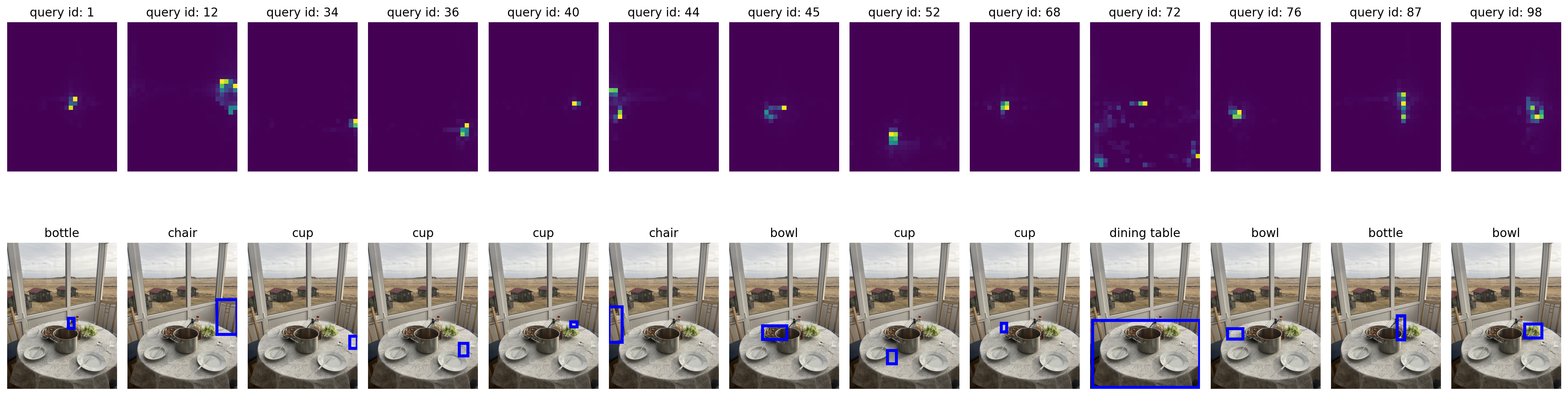
# output of the CNN
f_map = conv_features['0']
print("Encoder attention:      ", enc_attn_weights[0].shape)
print("Feature map:            ", f_map.tensors.shape)
위 코드는 CNN 출력과 인코더의 attention weight의 모양을 출력하여 모델이 생성한 feature map과 attention map의 구조를 확인하는 데 사용됩니다.
# get the HxW shape of the feature maps of the CNN
shape = f_map.tensors.shape[-2:]
# and reshape the self-attention to a more interpretable shape
sattn = enc_attn_weights[0].reshape(shape + shape)
print("Reshaped self-attention:", sattn.shape)
이 코드는 CNN feature map의 w, h를 얻고, 인코더의 self-attention 가중치를 보다 해석하기 쉬운 형태로 변환합니다.
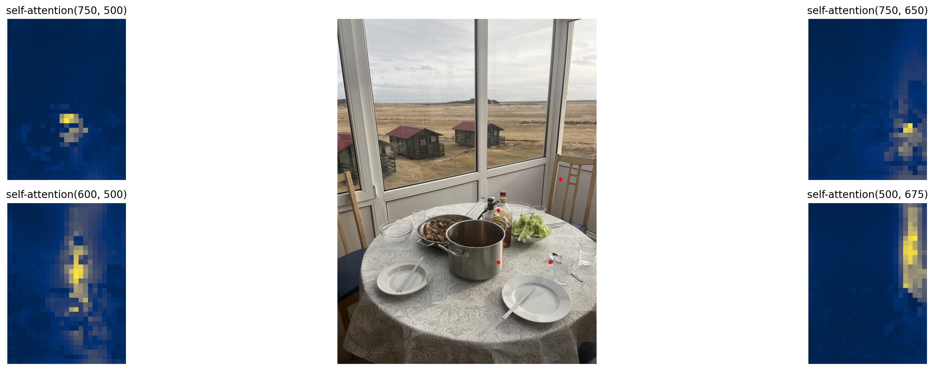
# downsampling factor for the CNN, is 32 for DETR and 16 for DETR DC5
fact = 32

# let's select 4 reference points for visualization
# dining table, bottle, cup, chair을 지정
idxs = [(750, 500), (600, 500), (750, 650), (500, 675)]

# here we create the canvas
fig = plt.figure(constrained_layout=True, figsize=(25 * 0.7, 8.5 * 0.7))
# and we add one plot per reference point
gs = fig.add_gridspec(2, 4)
axs = [
    fig.add_subplot(gs[0, 0]),
    fig.add_subplot(gs[1, 0]),
    fig.add_subplot(gs[0, -1]),
    fig.add_subplot(gs[1, -1]),
]

# for each one of the reference points, let's plot the self-attention
# for that point
for idx_o, ax in zip(idxs, axs):
    idx = (idx_o[0] // fact, idx_o[1] // fact)
    ax.imshow(sattn[..., idx[0], idx[1]], cmap='cividis', interpolation='nearest')
    ax.axis('off')
    ax.set_title(f'self-attention{idx_o}')

# and now let's add the central image, with the reference points as red circles
fcenter_ax = fig.add_subplot(gs[:, 1:-1])
fcenter_ax.imshow(im)
for (y, x) in idxs:
    scale = im.height / img.shape[-2]
    x = ((x // fact) + 0.5) * fact
    y = ((y // fact) + 0.5) * fact
    fcenter_ax.add_patch(plt.Circle((x * scale, y * scale), fact // 2, color='r'))
    fcenter_ax.axis('off')
위 코드를 통해 DETR 모델의 self-attention 가중치를 시각화하여, 모델이 이미지에서 주목한 영역을 나타낼 수 있습니다.
각각 dining table, bottle, cup, chair 순서로 reference point를 잡아 주목한 영역을 나타내보았습니다.