인공지능/Artificial Intelligence (COSE361)
[인공지능] Chapter 9. Markov Decision Process (1)
이준언
2023. 10. 25. 15:17
Markov Decision Processes
- 다음과 같은 요소로 정의
- A set of states s from S
- A set of actions a from A
- A transition function T(s, a, s’)
- s’: a(from s)가 s’가 될 확률
- Also called the model or the dynamic
- A reward function R(s, a, s’)
- A start stae
- Maybe a terminal state
- MDPs are non-deterministic search problems
- One way to solve them is with expectimax search
What is Markov about MDPs?
- Markov
- generally means that given the present state, the future and the past are independent (미래와 과거 상태가 조건적으로 독립)
- For Markov decision processes, ‘Markov’ means action outcomes depend only on the current state (action의 결과가 현재 상태에만 의존)
- 이는 successor function이 history가 아닌, current state에만 의존할 수 있는 검색과 유사
Policies
- In deterministic single-agent search problems,
- we wanted an optimal plan
- or sequence of actions, from start to a goal
- For MDPs, we want an optimal policy
- it gives an action for each state
- An optimal policy is one that maximizes expected utility if followed
- An explicit policy defines a reflex agent
- Expectimax didn’t compute entire policies
- It computed the action for a single state only
- Example: Racing
- A robot car wants to travel far, quickly
- states
- Cool
- Warm
- Overheated
- actions
- Slow
- Fast
- Going faster gets double reward
Discounting
- sum of rewards를 최대화하는 것이 바람직
- rewards later 보다 rewards now를 선호하는 것이 바람직
- One solution: values of rewards decay exponentially
- How to discount?
- level을 descend할 때마다, discount를 한 번 씩 곱함
- Why discount?
- 빠른 rewards는 나중에 받는 rewards보다 높은 utility를 갖는다.
- 알고리즘이 수렴하는 데에 도움이 된다.
Stationary Preferences
- Theorem
- If we assume stationary preferences:
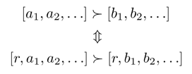
- Then there are only two ways to define utilities

- If we assume stationary preferences:
Infinite Utilities
- 문제
- 게임이 계속 지속되면 어떻게 되는가? 무한대의 reward를 받을 수 있는가?
- 해결
- Finite horizon (similar to depth-limited search)
- fixed T step 이후 episode 종료
- nonstationary police 제공
- Discounting
- use 0<γ<1

- Smaller γ means smaller ‘horizon’
- shorter term focus
- use 0<γ<1
- Absorbing state
- 모든 policy에 대해 종료상태에 도달하도록 보장
- Finite horizon (similar to depth-limited search)
Solving MDPs
- Optimal Quantities
- The value(utility) of a state s
- V*(s)
- expected utility starting in s and acting optimally
- V*(s)
- The value(utility) of a q-state (s, a)
- Q*(s, a)
- expected utility starting out having taken action a from state s and (thereafter) acting optimally
- Q*(s, a)
- The optimal policy
- 𝜋∗ (𝑠)
- optimal action from state 𝑠
- 𝜋∗ (𝑠)
- The value(utility) of a state s
- Values of States
- Fundamental operation (기본 연산)
- 각 상태의 expectimax value를 계산
- optimal action에 따른 expected utility
- rewards 합계의 평균
- expectimax 계산과 유사
- Fundamental operation (기본 연산)
- Racing Search Tree
- expectimax
- 문제1: 상태가 반복됨
- 필요한 수량을 한 번만 계산
- 문제2: Tree goes on forever
- 깊이 제한 계산을 수행하되, 변화가 작아질 때까지 깊이를 증가
- Time-Limited Values
- 𝑉_𝑘 (𝑠)
- optimal value of s
- if the game ends in k more time steps
- 즉, s에서 depth-k expectimax를 얻을 수 있는 값
- 𝑉_𝑘 (𝑠)
Value Iteration
- Value Iteration
- V_0(s) = 0 에서 시작
- no time steps left means an expected sum of reward = 0
- V_k(s)를 고려하면, 각 상태에서 expectimax를 한 번씩 수행
- 수렴 시까지 반복
- 각 반복의 복잡도: O(A * S^2)
- Theorem
- will converge to unique optimal values
- Basic idea: approximations get refined towards optimal values
- Policy may converge long before values do
Convergence
- How do we know the V_k vectors are going to converge?
- Case 1
- 트리의 최대 깊이가 M인 경우, V_M holds the actual untruncated values
- Case 2
- If the discount is less than 1
- Sketch: 어떤 상태에 대해 V_k와 V_(k+1)는 거의 동일한 검색트리에서 depth k+1 expectimax result로 볼 수 있음
- 차이점:
- 최하위 계층에서, V_(k+1)에는 실제 rewards가 있는 반면, V_k는 0이다.
- 마지막 레이어는 at best all R_max
- 최악의 경우 R_min
- But everything is discounted by 𝛾^𝑘
- Case 1
Summary
- MDP can model problems with uncertain outcomes of actions
- Solving an MDP is to find the optimal policy
- The optimal policy provides the optimal action to take at each state
- Q-states are introduced to model uncertainty in the outcomes of an action
- Values of states and q-values of q-states are defined recursively
- Values of states can be computed through the value iteration algorithm